Feature overview#
The following presents a descriptive example show-casing all core features of GeoUtils.
Tip
All pages of this documentation containing code cells can be run interactively online without the need of setting up your own environment. Simply click the top launch button! (MyBinder can be a bit capricious: you might have to be patient, or restart it after the build is done the first time 😅)
Alternatively, start your own notebook to test GeoUtils at ![]() .
.
The core Raster, Vector and PointCloud objects#
In GeoUtils, geospatial handling is object-based and revolves around Raster and Vector.
These link to either in-memory or on-disk datasets, opened by calling the object from a filepath for the latter.
import geoutils as gu

# Examples files: infrared band of Landsat and glacier outlines
filename_rast = gu.examples.get_path("everest_landsat_b4")
filename_vect = gu.examples.get_path("everest_rgi_outlines")

# Open files by calling Raster and Vector
rast = gu.Raster(filename_rast)
vect = gu.Vector(filename_vect)
A Raster is an object with four main attributes: a numpy.ma.MaskedArray as data, a
pyproj.crs.CRS as crs, an affine.Affine
as transform, and a float or int as nodata.
# The opened raster
rast
Raster(
  data=not_loaded; shape on disk (1, 655, 800); will load (655, 800)
  transform=| 30.00, 0.00, 478000.00|
            | 0.00,-30.00, 3108140.00|
            | 0.00, 0.00, 1.00|
  crs=EPSG:32645
  nodata=None)
Important
When a file exists on disk, Raster is linked to a rasterio.io.DatasetReader object for loading the metadata. The array will be
loaded in-memory implicitly when data is required by an operation.
See Implicit lazy loading for more details.
A Vector is an object with a single main attribute: a GeoDataFrame as ds, for which
most methods are wrapped directly into Vector.
# The opened vector
vect
Vector(
  ds=             RGIId         GLIMSId   BgnDate   EndDate     CenLon     CenLat  \
       0   RGI60-15.03410  G086932E27925N  20001030  -9999999  86.932083  27.924758
       1   RGI60-15.03411  G086939E27924N  20001030  -9999999  86.939035  27.923919
       2   RGI60-15.03412  G086852E27949N  20001030  -9999999  86.851810  27.948727
       3   RGI60-15.03413  G086848E27952N  20001030  -9999999  86.848051  27.951937
       4   RGI60-15.03414  G086849E27966N  20001030  -9999999  86.848799  27.966443
       ..             ...             ...       ...       ...        ...        ...
       81  RGI60-15.10070  G086956E28089N  20100409  -9999999  86.956000  28.089000
       82  RGI60-15.10075  G086960E28045N  20100409  -9999999  86.960000  28.045000
       83  RGI60-15.10077  G086963E28079N  20100409  -9999999  86.963000  28.079000
       84  RGI60-15.10078  G086966E28051N  20100409  -9999999  86.966000  28.051000
       85  RGI60-15.10079  G086969E28097N  20100409  -9999999  86.969000  28.097000

          O1Region O2Region    Area  Zmin  ...  Aspect  Lmax  Status  Connect  Form  \
       0        15        2   0.980  5196  ...     310  1184       0        0     0
       1        15        2   0.064  5831  ...      78   309       0        0     0
       2        15        2   0.059  5509  ...      29   269       0        0     0
       3        15        2   0.176  5400  ...     341   790       0        0     0
       4        15        2   0.477  5280  ...     284   845       0        0     0
       ..      ...      ...     ...   ...  ...     ...   ...     ...      ...   ...
       81       15        2  12.646  5940  ...     266  5413       0        0     1
       82       15        2   0.143  6530  ...     262   426       0        0     0
       83       15        2   0.051  6420  ...     307   395       0        0     0
       84       15        2   0.181  6559  ...     321   461       0        0     0
       85       15        2   0.136  6538  ...     203   571       0        0     0

           TermType  Surging  Linkages                               Name  \
       0          0        9         9                               None
       1          0        9         9                               None
       2          0        9         9                               None
       3          0        9         9                               None
       4          0        9         9                               None
       ..       ...      ...       ...                                ...
       81         0        9         9  CN5O193B0118 East Rongbuk Glacier
       82         0        9         9  CN5O193B0118 East Rongbuk Glacier
       83         0        9         9  CN5O193B0118 East Rongbuk Glacier
       84         0        9         9  CN5O193B0118 East Rongbuk Glacier
       85         0        9         9  CN5O193B0118 East Rongbuk Glacier

                                                    geometry
       0   POLYGON ((86.92842 27.92877, 86.92866 27.9293,...
       1   POLYGON ((86.94077 27.92375, 86.94059 27.92295...
       2   POLYGON ((86.85344 27.94752, 86.8534 27.94752,...
       3   POLYGON ((86.84776 27.94845, 86.84776 27.94849...
       4   POLYGON ((86.84567 27.96906, 86.84567 27.9691,...
       ..                                                ...
       81  POLYGON ((86.94112 28.11455, 86.94129 28.11452...
       82  POLYGON ((86.95861 28.04669, 86.95847 28.04701...
       83  POLYGON ((86.96454 28.07843, 86.96445 28.07814...
       84  POLYGON ((86.96302 28.04915, 86.96304 28.0492,...
       85  POLYGON ((86.97074 28.09496, 86.97039 28.09488...

       [86 rows x 23 columns]
  crs=EPSG:4326
  bounds=BoundingBox(left=np.float64(86.70393205700003), bottom=np.float64(27.847778695000045), right=np.float64(87.11409458600008), top=np.float64(28.14549759700003)))
All other attributes are derivatives of those main attributes, or of the filename on disk. Attributes of Raster and
Vector update with geospatial operations on themselves.
Handling and match-reference#
In GeoUtils, geospatial handling operations are based on class methods, such as crop() or reproject().
For convenience and consistency, nearly all of these methods can be passed solely another Raster or Vector as a
reference to match during the operation. A reference Vector enforces a matching of bounds and/or
crs, while a reference Raster can also enforce a matching of res, depending on the nature of the operation.
# Print initial bounds of the vector
print(vect.bounds)
# Crop vector to raster's extent, and add clipping option (otherwise keeps all intersecting features)
vect_cropped = vect.crop(rast, clip=True)
# Print bounds of cropped + clipped vector
print(vect_cropped.bounds)
BoundingBox(left=np.float64(86.70393205700003), bottom=np.float64(27.847778695000045), right=np.float64(87.11409458600008), top=np.float64(28.14549759700003))
BoundingBox(left=np.float64(86.77604281922927), bottom=np.float64(27.921168931302088), right=np.float64(87.02035980673882), top=np.float64(28.098736524870052))
Additionally, in GeoUtils, methods that apply to the same georeferencing attributes have consistent naming1 across Raster and Vector.
A reproject() involves a change in crs or transform, while a crop() only involves a change
in bounds. Using polygonize() allows to generate a Vector from a Raster,
and the other way around for rasterize().
Class |
||
|---|---|---|
Warping/Reprojection |
||
Cropping/Clipping |
||
Rasterize/Polygonize |
All methods can also be passed any number of georeferencing arguments such as shape or res, and will
naturally deduce others from the input Raster or Vector, much as in GDAL’s command line.
Higher-level analysis tools#
GeoUtils also implements higher-level geospatial analysis tools for both Rasters and Vectors. For
example, one can compute the distance to a Vector geometry, or to target pixels of a Raster, using
proximity().
As with the geospatial handling functions previously listed, many analysis functions can take a Raster or Vector as a
reference to utilize during the operation. In the case of proximity(), passing a Raster serves as a reference
for the georeferenced grid on which to compute the distances.
# Compute proximity to vector on raster's grid
rast_proximity_to_vec = vect.proximity(rast)
Note
Right now, the array data of rast is still not loaded. Applying crop() does not yet require loading,
and rast’s metadata is sufficient to provide a georeferenced grid for proximity(). The array will only be loaded when necessary.
Quick plotting#
To facilitate the analysis process, GeoUtils includes quick plotting tools that support multiple colorbars and implicitly add layers to the current axis.
Those are build on top of rasterio.plot.show() and geopandas.GeoDataFrame.plot(), and relay any argument passed.
See also
GeoUtils’ plotting tools only aim to smooth out the most common hassles when quickly plotting raster and vectors.
For advanced plotting tools to create “publication-quality” figures, see Cartopy or GeoPlot.
The plotting functionality is named plot() everywhere, for consistency. Here again, a Raster or
Vector can be passed as a reference to match to ensure all data is displayed on the same grid and projection.
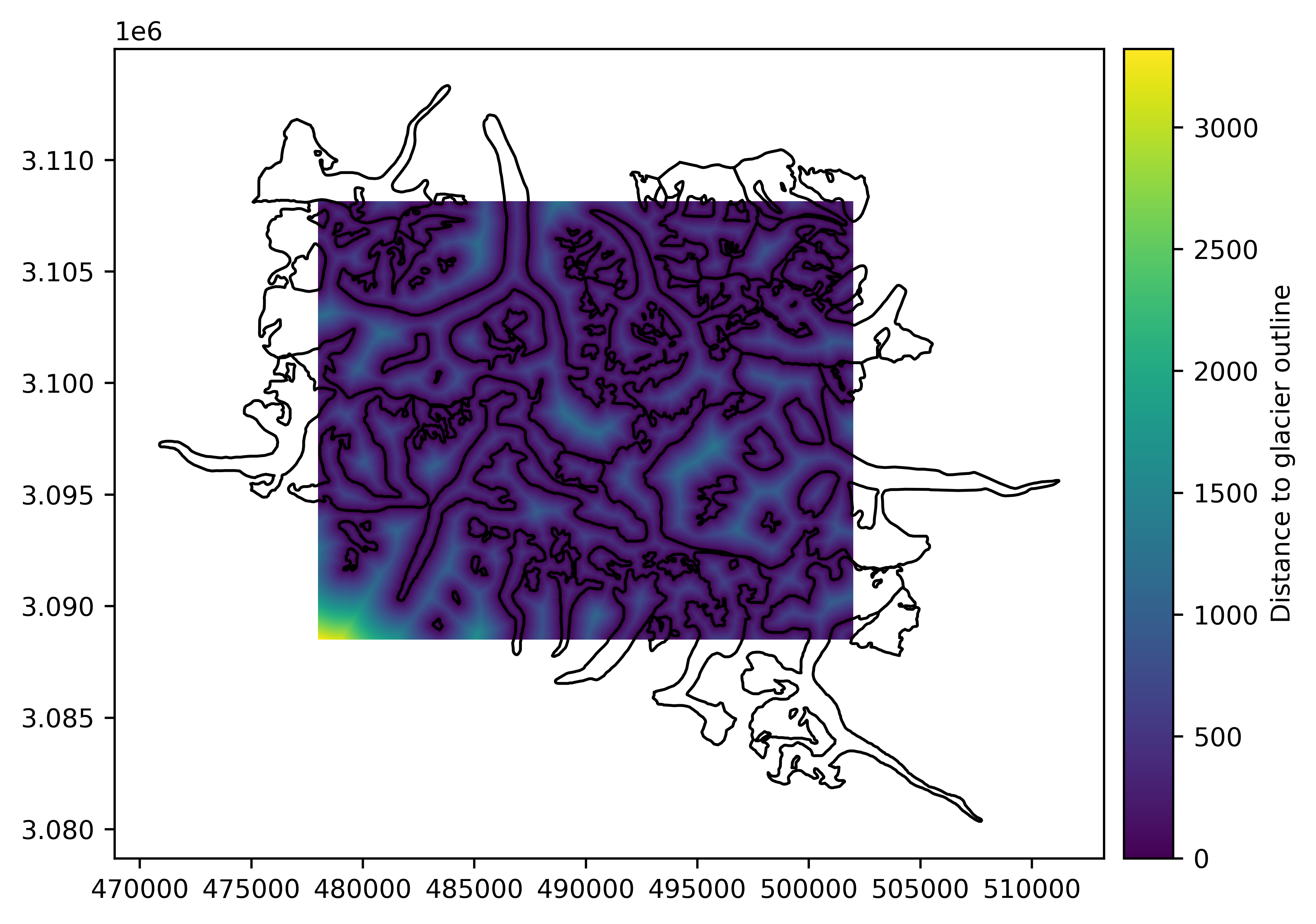
# Plot proximity to vector
rast_proximity_to_vec = vect.proximity(rast)
rast_proximity_to_vec.plot(cbar_title="Distance to glacier outline")
vect.plot(rast_proximity_to_vec, fc="none")
Tip
To quickly visualize a raster directly from a terminal, without opening a Python console/notebook, check out our tool geoviewer.py in the Command line interface documentation.
Pythonic arithmetic and NumPy interface#
All Raster objects support Python arithmetic (+, -, /, //, *,
**, %) with any other Raster, ndarray or
number. With another Raster, the georeferencing must match, while only the shape with a ndarray.
# Add 1 to the raster array
rast += 1
Additionally, the Raster object possesses a NumPy masked-array interface that allows to apply to it any NumPy universal function and
most other NumPy array functions, while logically casting dtype and respecting nodata values.
# Apply a normalization to the raster
import numpy as np
rast = (rast - np.min(rast)) / (np.max(rast) - np.min(rast))
Casting to raster mask, indexing and overload#
All Raster objects also support Python logical comparison operators (==, !=, >=, >, <=,
<), or more complex NumPy logical functions. Those operations automatically casts them into a raster mask, i.e. a boolean
Raster.
# Get mask of an AOI: infrared index above 0.6, at least 200 m from glaciers
mask_aoi = np.logical_and(rast > 0.6, rast_proximity_to_vec > 200)
Raster masks can then be used for indexing a Raster, which returns a MaskedArray of indexed values.
# Index raster with mask to extract a 1-D array
values_aoi = rast[mask_aoi]
Raster masks also have simplified Raster methods due to their boolean dtype rendering many arguments implicit.
For instance, using polygonize() with a raster mask is straightforward, to retrieve a Vector of the area-of-interest:
# Polygonize areas where mask is True
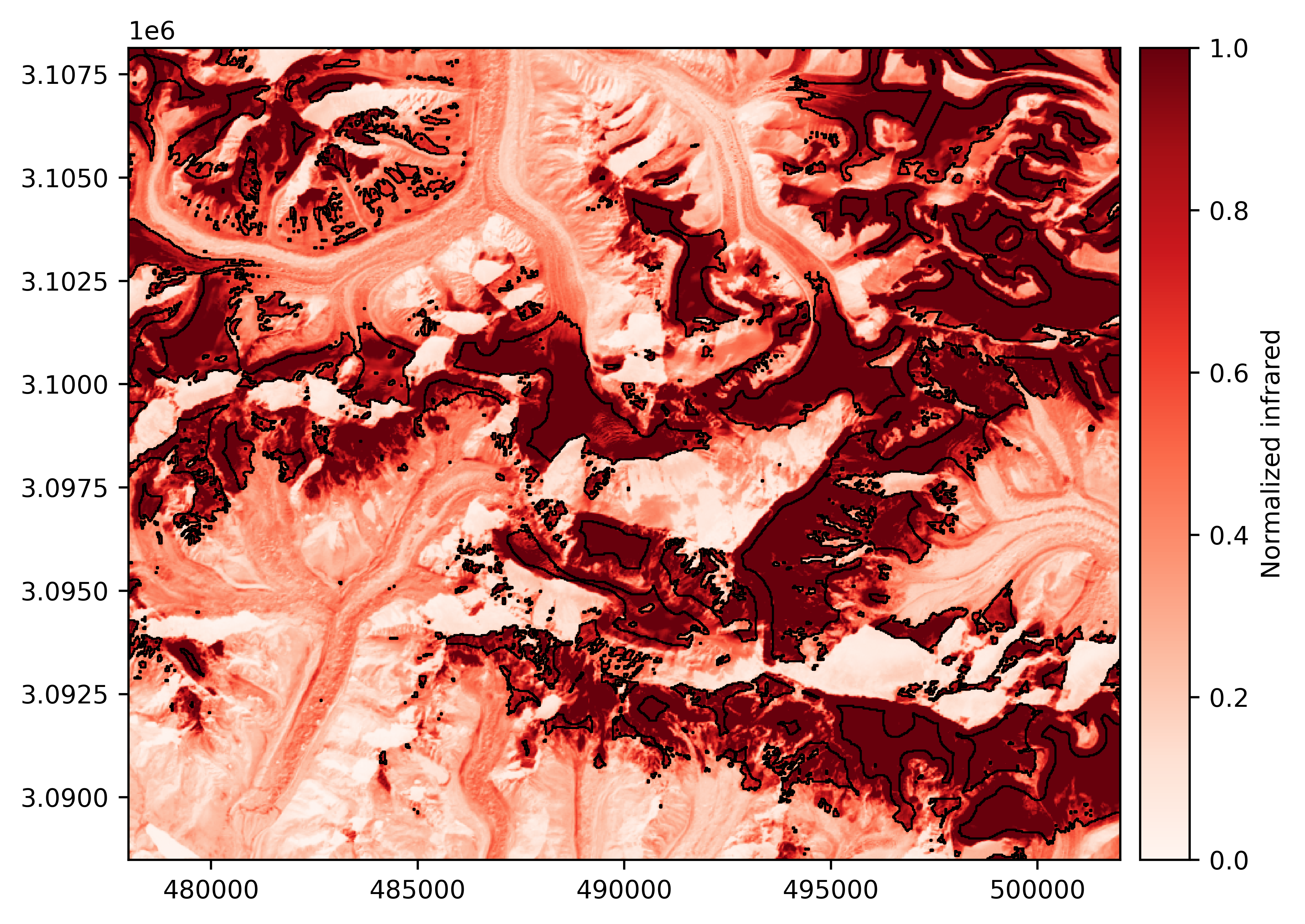
vect_aoi = mask_aoi.polygonize()
# Plot result
rast.plot(cmap='Reds', cbar_title='Normalized infrared')
vect_aoi.plot(fc='none', ec='k', lw=0.75)
Saving to file#
Finally, for saving a Raster or Vector to file, simply call the to_file() function.
# Save our AOI vector
vect_aoi.to_file("myaoi.gpkg")
Parsing sensor metadata#
In our case, rast would be better opened using the parse_sensor_metadata argument of a Raster,
which tentatively parses metadata recognized from the filename or auxiliary files.
# Name of the image we used
import os
print(os.path.basename(filename_rast))
LE71400412000304SGS00_B4.tif
# Open while parsing metadata
rast = gu.Raster(filename_rast, parse_sensor_metadata=True, silent=False)
Setting platform as Landsat 7 read from filename.
Setting sensor as ETM+ read from filename.
Setting tile_name as 140041 read from filename.
Setting datetime as 2000-10-30 00:00:00 read from filename.
Wrap-up
In a few lines, we:
easily handled georeferencing operations on rasters and vectors,
performed numerical calculations inherently respecting invalid data,
casted to a mask implicitly from a logical operation on raster, and
vectorized a mask without need for any additional metadata, simply using the nature of the mask object!
Our result: a vector of high infrared absorption indexes at least 200 meters away from glaciers near Everest, which likely corresponds to perennial snowfields.
Otherwise, for more hands-on examples, explore GeoUtils’ gallery of examples!