Raster–vector–point interface

GeoUtils provides functionalities at the interface of rasters, vectors and point clouds, allowing to consistently perform operations such as mask creation or point interpolation respecting both georeferencing and nodata values, as well as pixel interpretation for point interfacing.

Raster–vector operations

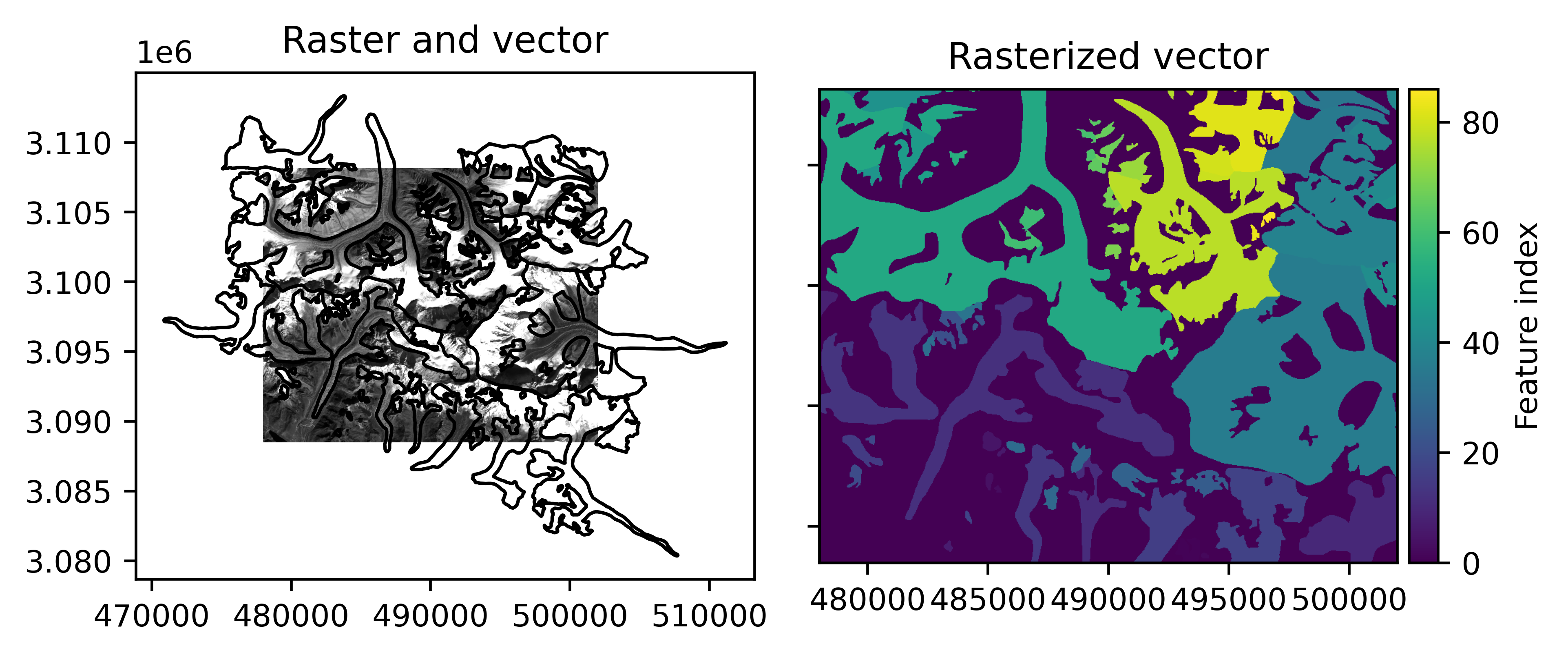
Rasterize

geoutils.Vector.rasterize()

Rasterization of a vector is an operation that allows to translate some information of the vector data into a raster, by setting the values raster pixels intersecting a vector geometry feature to that of an attribute of the vector associated to the geometry (e.g., feature ID, area or any other value), which is the geometry index by default.

Rasterization generally implies some loss of information, as there is no exact way of representing a vector on a grid. Rather, the choice of which pixels are attributed a value depends on the amount of intersection with the vector geometries and so includes several options (percent of area intersected, all touched, etc).

Show the code for opening example files

Hide the code for opening example files

import matplotlib.pyplot as plt
import geoutils as gu
import numpy as np

rast = gu.Raster(gu.examples.get_path("everest_landsat_b4"))
rast.set_nodata(0)  # Annoying to have to do this here, should we update it in the example?
vect = gu.Vector(gu.examples.get_path("everest_rgi_outlines"))

# Rasterize the vector features based on their glacier ID number
rasterized_vect = vect.rasterize(rast)

Show the code for plotting the figure

Hide the code for plotting the figure

f, ax = plt.subplots(1, 2)
ax[0].set_title("Raster and vector")
rast.plot(ax=ax[0], cmap="gray", add_cbar=False)
vect.plot(ref_crs=rast, ax=ax[0], ec="k", fc="none")
ax[1].set_title("Rasterized vector")
rasterized_vect.plot(ax=ax[1], cmap="viridis", cbar_title="Feature index")
_ = ax[1].set_yticklabels([])
plt.tight_layout()

Create mask

geoutils.Vector.create_mask()

Raster mask creation from a vector is a rasterization of all vector features that only categorizes geometry intersection as a boolean mask (if any feature falls in a given pixel or not), and is therefore independent of any vector attribute values.

# Create a boolean mask from all vector features
mask = vect.create_mask(rast)

Show the code for plotting the figure

Hide the code for plotting the figure

f, ax = plt.subplots(1, 2)
ax[0].set_title("Raster and vector")
rast.plot(ax=ax[0], cmap="gray", add_cbar=False)
vect.plot(ref_crs=rast, ax=ax[0], ec="k", fc="none")
ax[1].set_title("Mask from vector")
mask.plot(ax=ax[1], cbar_title="Intersects vector (1=yes, 0=no)")
_ = ax[1].set_yticklabels([])
plt.tight_layout()

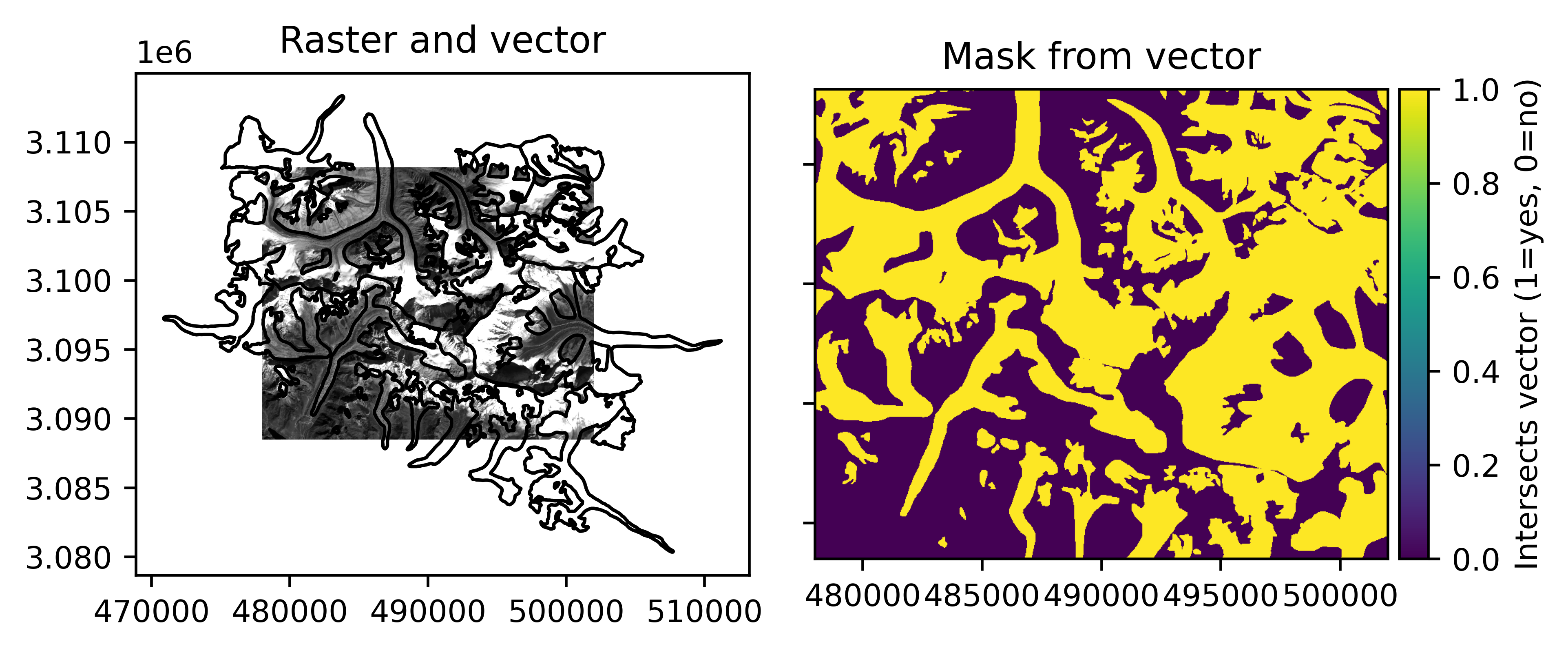
It returns a raster mask, a georeferenced boolean Raster (or optionally, a boolean NumPy array), which can both be used for indexing or index assignment of a raster.

# Mean of values in the mask
np.mean(rast[mask])

np.float64(172.66101371277432)

Polygonize

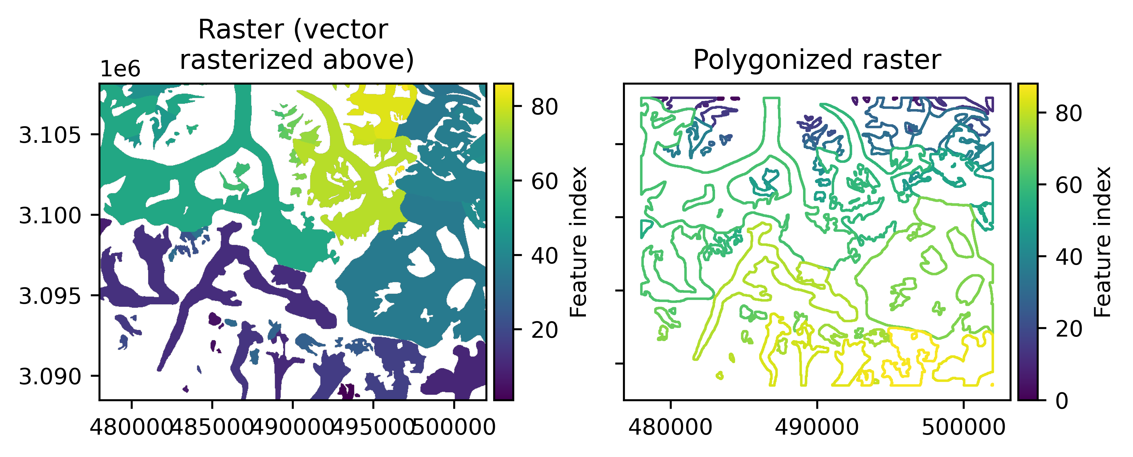
geoutils.Raster.polygonize()

Polygonization of a raster consists of delimiting contiguous raster pixels with the same target values into vector polygon geometries. By default, all raster values are used as targets. When using polygonize on a raster mask, i.e. a boolean Raster, the targets are implicitly the valid values of the mask.

# Mask 0 values
rasterized_vect.set_mask(rasterized_vect == 0)
# Polygonize all non-zero values
vect_repolygonized = rasterized_vect.polygonize()

Show the code for plotting the figure

Hide the code for plotting the figure

f, ax = plt.subplots(1, 2)
ax[0].set_title("Raster (vector\n rasterized above)")
rasterized_vect.plot(ax=ax[0], cmap="viridis", cbar_title="Feature index")
ax[1].set_title("Polygonized raster")
vect_repolygonized.plot(ax=ax[1], column="id", fc="none", cbar_title="Feature index")
_ = ax[1].set_yticklabels([])
plt.tight_layout()

Raster–point operations

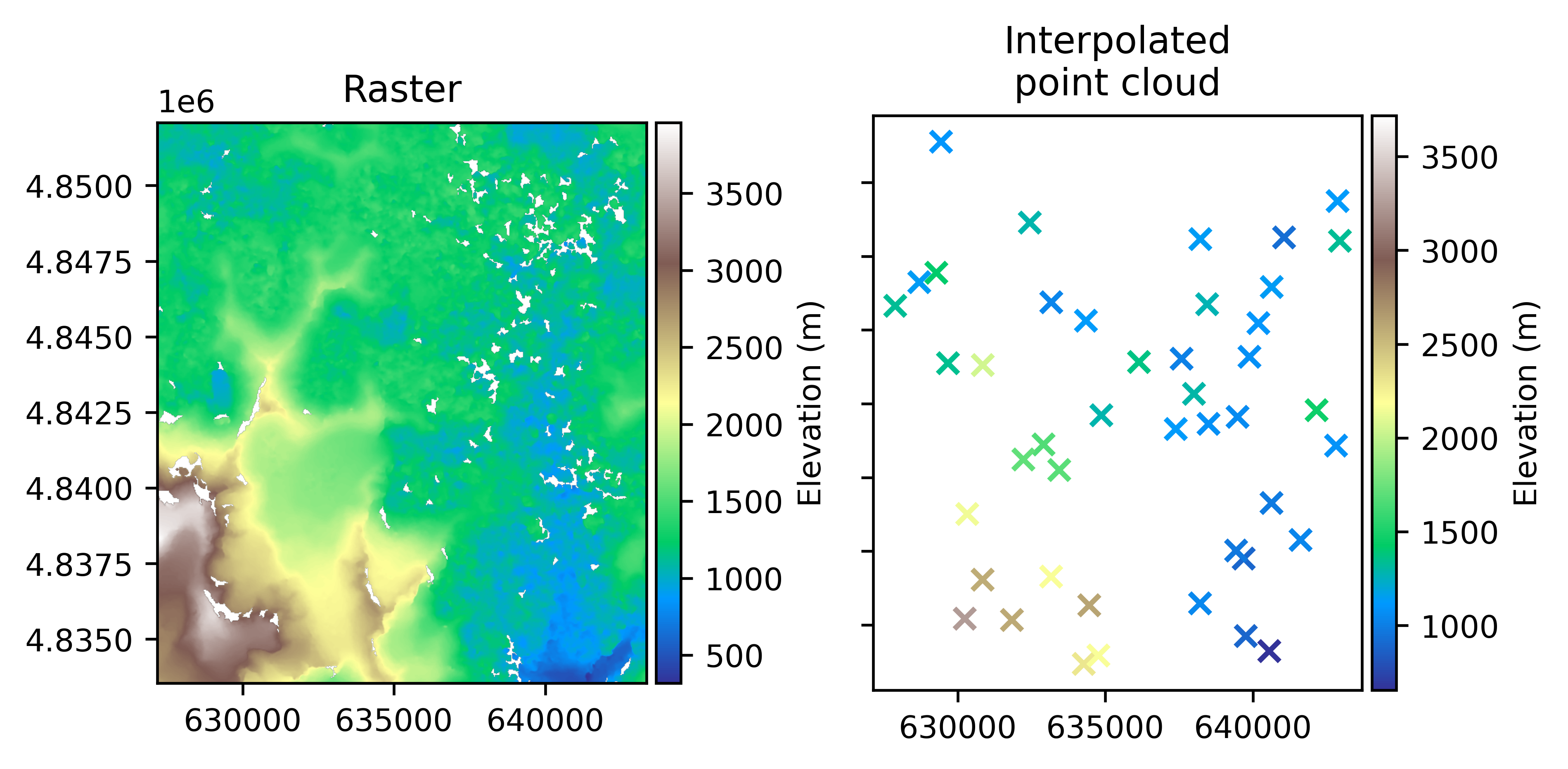
Point interpolation

geoutils.Raster.interp_points()

Point interpolation of a raster consists in estimating the values at exact point coordinates by 2D regular-grid interpolation such as nearest neighbour, bilinear (default), cubic, etc.

Note

In order to support all types of resampling methods with nodata values while maintaining the robustness of results, GeoUtils implements a modified version of scipy.interpolate.interpn() that propagates nodata values in surrounding pixels of initial nodata values depending on the order of the resampling method:

• Nearest or linear (order 0 or 1): up to 1 pixel,

• Cubic (order 3): 2 pixels,

• Quintic (order 5): 3 pixels.

# We use a DEM, often requiring interpolation
rast =  gu.Raster(gu.examples.get_path("exploradores_aster_dem"))

# Get 50 random points to sample within the raster extent
rng = np.random.default_rng(42)
x_coords = rng.uniform(rast.bounds.left, rast.bounds.right, 50)
y_coords = rng.uniform(rast.bounds.bottom, rast.bounds.top, 50)

pc_int = rast.interp_points(points=(x_coords, y_coords))

The interpolated points can be returned as a PointCloud, enabling quick interfacing, or as an array.

Show the code for plotting the figure

Hide the code for plotting the figure

f, ax = plt.subplots(1, 2)
ax[0].set_title("Raster")
rast.plot(ax=ax[0], cmap="terrain", cbar_title="Elevation (m)")
ax[1].set_title("Interpolated\npoint cloud")
pc_int.plot(ax=ax[1], cmap="terrain", cbar_title="Elevation (m)", marker="x")
_ = ax[1].set_yticklabels([])
plt.tight_layout()

Reduction around point

Point reduction of a raster is the estimation of the values at point coordinates by applying a reductor function (e.g., mean, median) to pixels contained in a window centered on the point. For a window smaller than the pixel size, the value of the closest pixel is returned.

geoutils.Raster.reduce_points()

pc_red = rast.reduce_points((x_coords, y_coords), window=5, reducer_function=np.nanmedian)

The reduced points can be returned as a PointCloud, enabling quick interfacing, or as an array.

Show the code for plotting the figure

Hide the code for plotting the figure

f, ax = plt.subplots(1, 2)
ax[0].set_title("Raster")
rast.plot(ax=ax[0], cmap="terrain", cbar_title="Elevation (m)")
ax[1].set_title("Reduced\npoint cloud")
pc_red.plot(ax=ax[1], cmap="terrain", cbar_title="Elevation (m)")
_ = ax[1].set_yticklabels([])
plt.tight_layout()

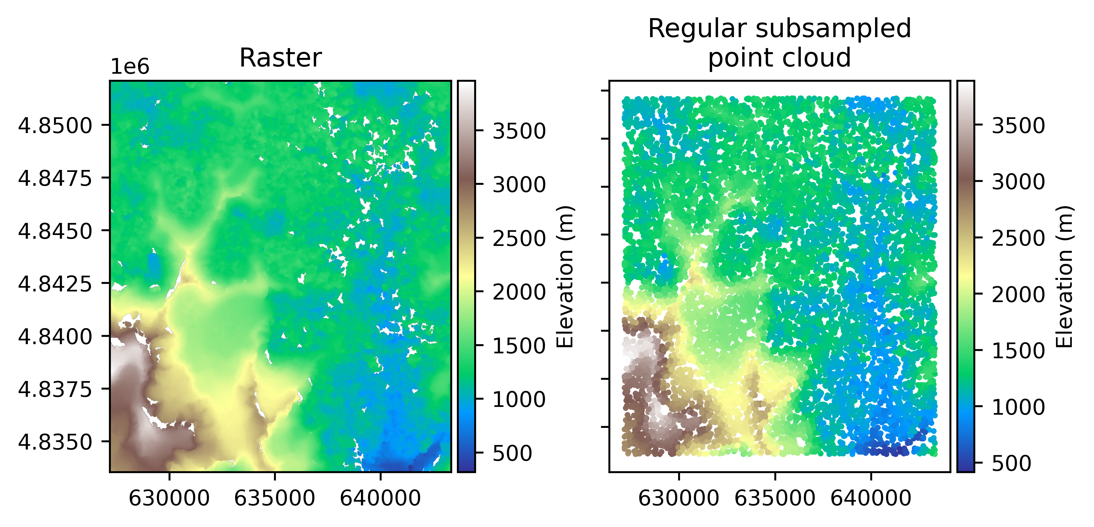
Raster to points

geoutils.Raster.to_pointcloud()

A raster can be converted exactly into a point cloud, which each pixel in the raster is associated to its pixel values to create a point cloud on a regular grid.

pc = rast.to_pointcloud(subsample=10000)

Show the code for plotting the figure

Hide the code for plotting the figure

f, ax = plt.subplots(1, 2)
ax[0].set_title("Raster")
rast.plot(ax=ax[0], cmap="terrain", cbar_title="Elevation (m)")
ax[1].set_title("Regular subsampled\npoint cloud")
pc.plot(ax=ax[1], cmap="terrain", cbar_title="Elevation (m)", markersize=2)
_ = ax[1].set_yticklabels([])
plt.tight_layout()

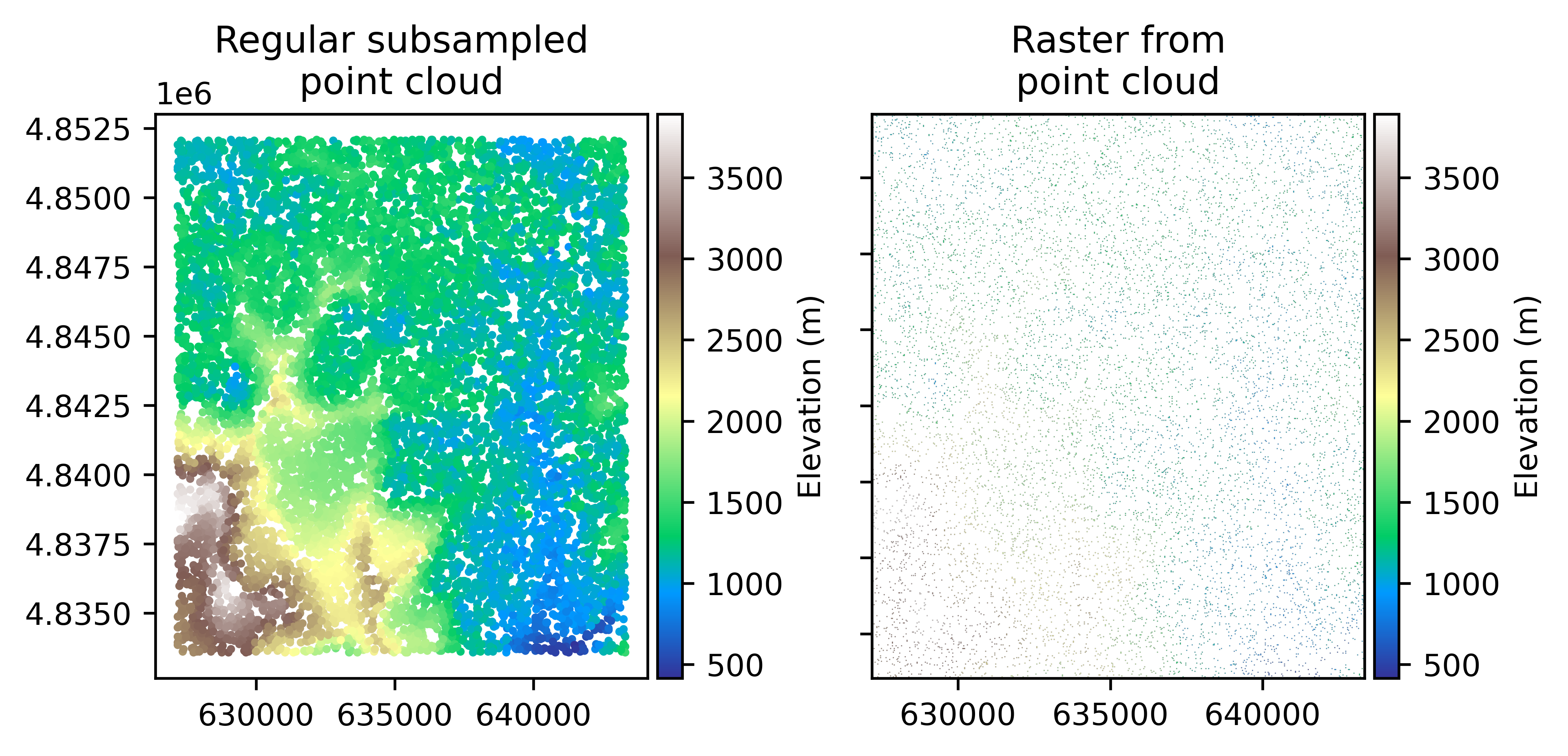
Regular points to raster

geoutils.Raster.from_pointcloud_regular()

If a point cloud is regularly spaced in X and Y coordinates, it can be converted exactly into a raster. Otherwise, it must be re-gridded using Point gridding described below. For a regular point cloud, every point is associated to a pixel in the raster grid, and the values are set to the raster. The point cloud does not necessarily need to contain points for all grid coordinates, as pixels with no corresponding point are set to nodata values.

rast_from_pc = gu.Raster.from_pointcloud_regular(pc, transform=rast.transform, shape=rast.shape)

Show the code for plotting the figure

Hide the code for plotting the figure

f, ax = plt.subplots(1, 2)
ax[0].set_title("Regular subsampled\npoint cloud")
pc.plot(ax=ax[0], cmap="terrain", legend=True, cbar_title="Elevation (m)", markersize=2)
ax[1].set_title("Raster from\npoint cloud")
rast_from_pc.plot(ax=ax[1], cmap="terrain", cbar_title="Elevation (m)")
_ = ax[1].set_yticklabels([])
plt.tight_layout()

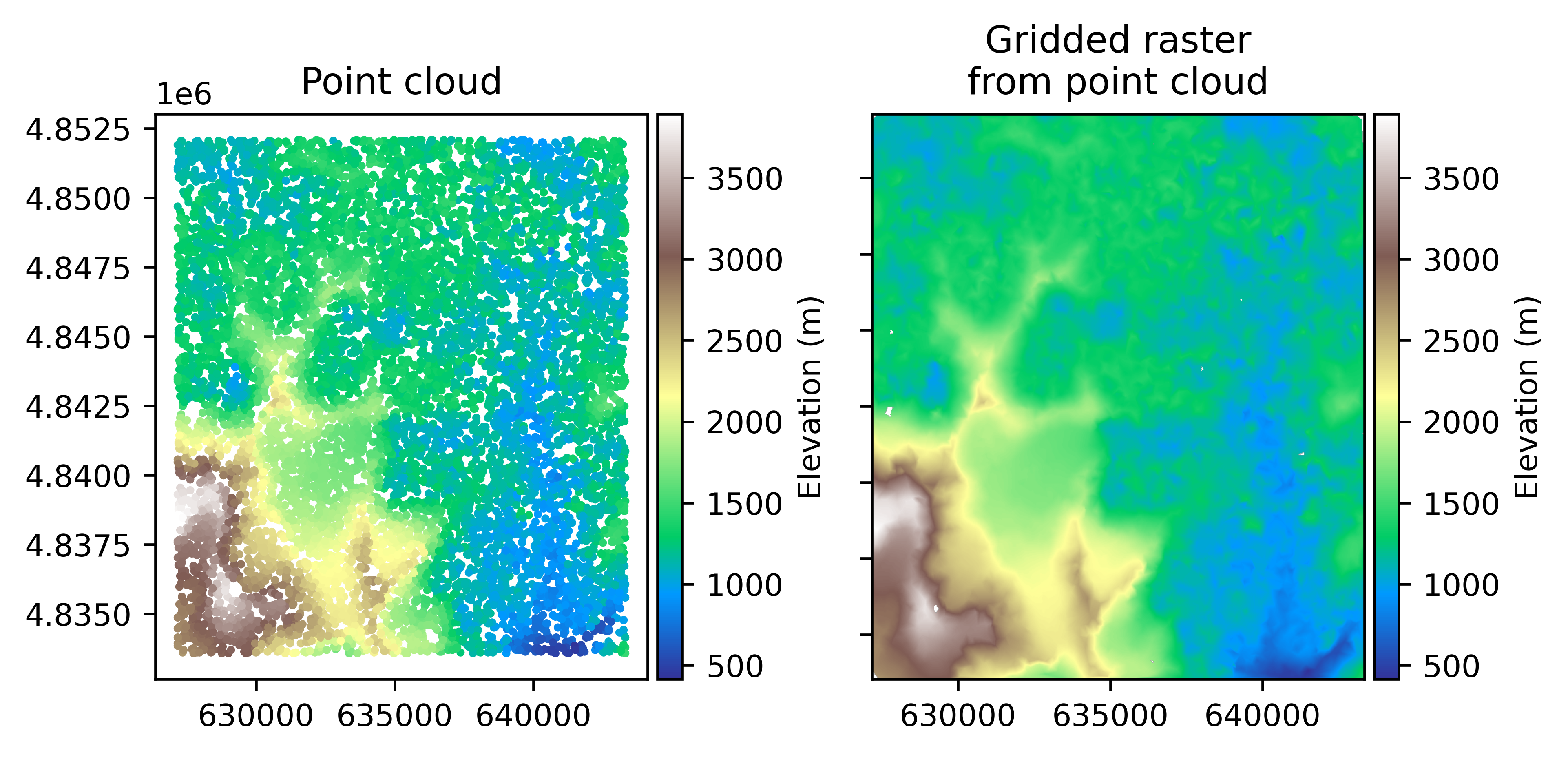
Point gridding

Gridding of a point cloud consists in estimating the values at 2D regular gridded coordinates based on an irregular point cloud using Delauney triangular interpolation (default), inverse-distance weighting or kriging.

Note

For gridding, GeoUtils introduces nodata values in distances surrounding initial point coordinates, defaulting to a distance of 1 pixel.

geoutils.PointCloud.grid()

# Grid points with raster as reference, add nodata only 10 pixels away from points
gridded_pc = pc.grid(rast, dist_nodata_pixel=10)

Show the code for plotting the figure

Hide the code for plotting the figure

f, ax = plt.subplots(1, 2)
ax[0].set_title("Point cloud")
pc.plot(ax=ax[0], cmap="terrain", legend=True, cbar_title="Elevation (m)", markersize=2)
ax[1].set_title("Gridded raster\nfrom point cloud")
gridded_pc.plot(ax=ax[1], cmap="terrain", cbar_title="Elevation (m)")
_ = ax[1].set_yticklabels([])
plt.tight_layout()